The Natural Refrigeration

CFD-based Design Basis for Avoidance of Hydraulic Shock in Ammonia Pipework Systems

Author:
Chidambaram Narayanan, Principal Engineer AFRY Switzerland AG

Abstract

Incidents of ammonia releases due to hydraulic shock in the refrigeration pipework have been reported in the past and could occur in the future. Such shock events carry significant commercial risks and are a concern for the health and safety of humans. Two locations where hydraulic shock occurs frequently are, (a) in the evaporator coil headers at the beginning of a hot gas defrost sequence, and (b) in the wet suction piping from the evaporator at the end of the hot gas defrost sequence. Research on experimental and numerical characterization of hydraulic shocks in ammonia systems was carried out through two impactful projects funded by ASHRAE. In the latter project a validated CFD model was developed using the experimental data as a basis. This CFD model was subsequently applied to a real incident where a shock amplitude of 4,000 psia was predicted as expected from forensic analysis. The validated CFD model was used in this study to simulate a large set of conditions related to generic hot gas defrost piping, to establish a design basis prevent hydraulic shock.

The parametric study consisted of 164 three-dimensional, unsteady simulations for a generic horizontal test pipe configuration and a set of initial conditions. Simulations were run for 2”, 4”, and 6” pipes with different lengths, liquid levels, evaporation temperatures and hot gas flow rates. A correlation for the shock amplitude for fast acting valves was developed as a function of operating conditions. This correlation can be directly used to assess the hydraulic shock risk in current refrigeration systems with single or two step fast-acting valves. The critical mass flow rate correlation which gives an upper limit on the mass flow rate for fast acting valves if hydraulic shocks are to be prevented is presented. Simulations of motorized valves for different opening times have shown that valve opening times greater than the system length divided by the average slug velocity will significantly reduce the shock pressures. This time scale can be directly estimated from the correlation developed in this study for the shock amplitude as a function of operating conditions. Based on these results, this study can lay the foundation for new design guidelines in the future.

Introduction

Incidents of ammonia releases due to hydraulic shock are still occurring. A welldocumented failure of an 8″ evaporator coil header operating at -50°F in an ammonia system serving a spiral freezer in a frozen food factory is presented by Wiencke (Wiencke, 2008). Under the best-case scenario, a hydraulic shock that causes a mechanical failure results in downtime for a plant. Larger shocks result in downtime, plus product loss, plus health effects to plant personnel, and neighboring communities. Two locations where hydraulic shocks occur most frequently are, (a) in the evaporator coil headers at the beginning of a hot gas defrost sequence, and (b) in the wet suction piping leaving the evaporator at the end of the hot gas defrost sequence.

Background

Condensation induced hydraulic shock (CIHS) occurs when there is accumulated or stratified liquid flowing in the piping, over which or behind which vapor at high velocity is introduced during a pressure transient. For a horizontal pipe partially filled with liquid, there is a shearing force of the gas acting on the gas-liquid interface. The interface forms waves which eventually grow to form slugs covering the full crosssection of the pipe. Further flow of vapor upstream pushes the slug toward a pipe end closure. As the trapped vapor gets pressurized, it condenses onto the oncoming slug and on the pipe walls. Thus, the slug does not experience any resistance to its motion and eventually collides with the end closure resulting in a hydraulic shock due to rapid collapse/condensation of the trapped gas. The shock pressures that are generated are commonly much higher than the maximum allowable working pressure of the low side of a refrigeration piping system and/or the setting of the pressure relief safety valves installed and designed to protect the system. It can now be confirmed through CFD modelling that these high-peak-pressure, short-duration, hydraulic shock pressure waves can exceed the strength of common low temperature ammonia refrigeration system piping. In addition, the transient pressure amplitude only exists for a very short duration and are very localized. If a pressure relief device would be installed close to the location where the shock event occurs, the short duration of the pressure rise would be too fast for the pressure relief valve to respond.

Martin et al. (Martin, Brown, & Brown, 2007) built a test rig around a 20-ft long, 6-inch schedule 80 pipe section that was fully instrumented to capture a hydraulic shock event. Slug formation, slug velocity and shock pressure were measured for 292 individual test runs over a period of eight months. Mass flow rates were varied so that thresholds for the occurrence of shocks were established at different initial void fractions. For the first time an extensive database of hydraulic shock data was available. To carry this research forward, the ASHRAE project RP-1569 was initiated in 2015 to develop and validate a CFD model based on the experimental data. The compressible, non-equilibrium, multiphase flow CFD model in TransAT (Labois & Narayanan, 2017) was developed further to gain the ability to simulate the CIHS problem and applied to the dataset of Martin et al. (Martin, Brown, & Brown, 2007). The study resulted, to the authors knowledge, in the first successful threedimensional CFD simulation of the CIHS phenomenon (Narayanan, Thomas, & Lakehal, CFD Study of Hydraulic Shock in Two-Phase Anhydrous Ammonia, 2020). Some of the shock pressure oscillations obtained from the simulation were strikingly similar to the experimental results. Slug speeds, shock formation times, and shock amplitudes were predicted with reasonable accuracy for a variety of liquid depths, temperatures and vapor flow rates. The model confirmed the direct correlation between slug formation in the horizontal test pipe and the creation of a hydraulic shock.

This CFD model was then applied to an incident described in detail by Wiencke (Wiencke, 2008), wherein the cause for the pipework failure was attributed to a massive hydraulic shock (~4,000 psia) during the hot gas defrost cycle for a postulated condition of the evaporator load. The model predicted a hydraulic shock of 3,600 psia for this case, which was much beyond the experimental range of Martin et al. (2007), thereby demonstrating the relevance and utility of the CFD model to real industrial systems. These results were presented in Narayanan et al. (Narayanan, Wiencke, & Loyko, 2021).

Objective

For the first time a verified and validated CFD software is available for the ammonia refrigeration industry such that it can be used to quantitatively predict the formation and amplitudes of hydraulic shocks (Narayanan, Thomas, & Lakehal, 2020). The objective of present work was to develop a design basis for hot gas and wet suction pipework and valve group systems based on quantitative analysis of different design configurations. As per the state of the art, such decisions are typically made using rules of thumb and experience and this simulation study attempts to put such heuristic rules on a firm footing. The study presents estimates of the critical mass flow rates for single-step and two-step fast acting valves below which the formation of a liquid slug is hindered, provides a correlation to calculate the shock amplitude in a given piping system under given hot gas operating conditions, and also provides an estimate of the minimum opening times of motorized valves that minimize the risk of hydraulic shock.

Mathematical and Numerical Modelling

The mathematical model used in this study is the compressible non-equilibrium multiphase mixture model (Saurel & Lemetayer, 2001) where each phase has separate equation of state such that the phases can be superheated or subcooled. The detailed mathematical formulation is presented in Labois and Narayanan (Labois & Narayanan, 2017) and further details regarding its ability to model liquid slug formation, vapor propulsion, and condensation models is available in Narayanan et al. (Narayanan, Thomas, & Lakehal, 2020). Turbulence is modelled using the mixture Reynolds averaged Navier-Stokes (RANS) approach. 

Two-phase Homogeneous Mixture Model

For multiphase flow problems, two different numerical techniques are available. The Interface Tracking Method is exclusively used for two-phase flows where the interface between the two fluids is sharp, and its evolution is to be tracked. The second technique is the mixture model where the two-phases can be separated or get mixed depending on the flow conditions and a clear interface between the vapor and liquid phases is not always available. In the compressible two-phase homogeneous mixture model used in this study (Labois & Narayanan, 2017), the conservation of mass equations are solved for each phase, whereas the momentum, pressure, and temperature are solved only for the mixture.

Condensation Modelling

Condensation controls two critical aspects of the CIHS problem. On one hand, vapor flow into a closed system results in a pressure rise and reduction in the velocity of the vapor. This hinders the formation of a liquid slug. At the same time, even if a slug is formed, the process of creation of a hydraulic shock depends on the propulsion of the liquid slug due to condensation of the trapped gas pocked downstream of the slug leading to its eventual collapse. Therefore, sufficiently accurate modelling of condensation is necessary to predict the formation of a hydraulic shock.

Phase change (boiling and condensation) phenomena can be broadly categorized as thermally limited and inertial phase change. Thermally limited phase change occurs when the temperature departs from the saturation condition whereas pressure is constant in the system (typically when heat is introduced or removed from a system). Within the thermally limited category, condensation can occur via several different mechanisms or modes, such as interfacial condensation, dispersed-phase condensation, and wall condensation. Inertial phase change happens when the pressure changes rapidly whereas the temperature varies less and is referred to as cavitation or flashing. Cavitation or flashing models are required for situations of turning liquid flows or for cases of depressurization.

In the original study (Narayanan, Thomas, & Lakehal, 2020), the dispersed-phase condensation model was found to be sufficient. However, depending on the pipework configuration, cavitation modelling could be necessary to successfully consider movement of a liquid slug through pipe bends and elbows. The cavitation model also comes into play during the last stages of the formation of a hydraulic shock due to the rapid collapse of the trapped gas/bubble. In the present study, both the thermally limited and inertia-limited (cavitation/flashing) models were used.

Numerical Modelling

The model is implemented into TransAT© software which is a finite-volume CFD solver specialized in the modelling of multiphase flows. The convective terms in the momentum and phasic continuity equations are discretized using the second order HLPA scheme (Zhu, 1991), whereas in the pressure equation the first-order upwind scheme is employed. The diffusion terms are discretized by second-order central differencing in the momentum and temperature equations. The pressure equation is solved using the SIMPLEC pressure correction method (Van Doormaal & Raithby, 1984). First-order backward Euler time stepping is used for the unsteady problems presented here. The compressibility of the two-phase system is modeled using pressure-based method developed by Labois & Narayanan (Labois & Narayanan, 2017). The local densities of each phase are calculated from the equation of state, ρk=ρk(T,p), where k denotes the phase. The conservation of mass equations for both phases are solved because, in general, the continuous phase can change in different regions of the flow. The volume fraction constraint Σαk=1, is maintained by consistent discretization and by subtracting the mixture continuity equation from each of the discrete phasic mass conservation equations.

Material and Transport Properties

In this multiphase flow model, each phase has a separate equation of state (EOS), and phases can be in metastable states, i.e., superheated liquid, and subcooled vapor. The fluid progresses towards equilibrium through phase-change source terms. The liquid density is estimated using the modified Tait EOS, whereas the vapor density is estimated using the Ideal gas EOS. Apart from the density, the simulation of the CIHS problem requires the specification of the latent heat of vaporization/condensation, the saturation curve, and the estimation of the speed of sound for both phases (available through the EOS). All the data used in this study has been compared with data available in the NIST Database for Ammonia. More details are available in Narayanan et al. (Narayanan, Thomas, & Lakehal, 2020).

Problem Setup

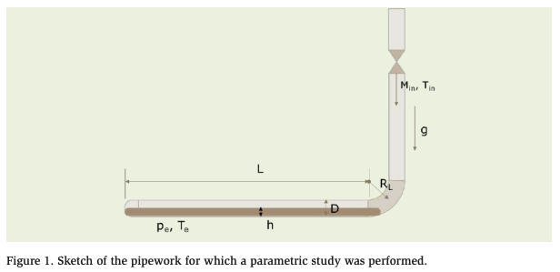
The geometry and setup for the first step is shown in Figure 1. A generic pipework, i.e., a horizontal pipe with hot gas entering through a smooth elbow, was chosen not only for the simplicity of analysis but also because the shock amplitudes could be higher in such a scenario. The flow problem is governed by three geometry parameters given by, the pipe diameter (D), the length of the horizontal part of the pipe (L), and the radius of the elbow (RL). However, the elbow radius was not considered in this study and was fixed to a value that is typically used in the industry (1.5 D). The parameters controlling the flow are the height of the liquid in the pipe (h), the evaporation pressure and temperature (pe, Te), the inlet hot-gas mass flow rate (Min), and hot-gas temperature (Tin).

Apart from the geometric and flow parameters, the fluid parameters also control the flow dynamics. A total of five fluid properties are required to be specified by the governing equations. These parameters are, the density, viscosity, thermal conductivity, heat capacity and the speed of sound for each phase. Additionally, the saturation curve of ammonia along with the variation of the latent heat along this curve is necessary. In summary, the problem is defined by 7 geometric and process parameters, and additionally the material and transport properties of Ammonia as a function of thermodynamic parameters, i.e., pressure and temperature. In arriving at the list of parameters the following assumptions were made:

1. The hot-gas valve remains choked (critical) during the process of hot gas defrost process under consideration; implying that the mass flow rate of hot gas will remain constant and not depend on the internal pressure in the pipework, and that
2. The valve discharge is represented using Min and Tin, which means that we have a transfer function that relates the upstream gas pressure and the valve size to these parameters.

The simulation domain was discretized by mesh size of 0.26″ across the cross-section for the 4″ pipe and 0.39″ mesh size for the 6″ pipe. This base mesh size was based on previous studies where they were found to be adequate (Narayanan, Thomas, & Lakehal, 2020). For select cases, simulations with a finer mesh (0.13″) were performed to ascertain that the results were not strongly dependent on the mesh.

Fast Acting Valves

The study first considered the situation of fast acting/instantaneous valves representing the opening of a regular solenoidal valve or the first step of a two-step solenoidal valve. The objective of this part is the predict the shock amplitudes as a function of the process parameters to aid in the design of valve groups. The analysis of motorized valves is presented in the next section.

A large set of simulations were performed using the CFD model in order to characterize the risk of a hydraulic shock for the first configuration shown in Figure 1. In total, 164 three-dimensional, unsteady, compressible, two-phase flow simulations with heat and mass transfer were run for characterizing instantaneous valves. Out of these, the first parametric study consisted of 96 cases, followed by additional simulations that will be described in the following sections. However, before the simulations were performed the modelling approach was revisited to make sure that it gave reliable results. Additionally, as a post processing tool, a slug detection algorithm was implemented to extract more information from each of the simulations.

Model Evaluation

Before launching a large parametric study consisting of three-dimensional unsteady simulations the model parameters were analyzed, and an acceptable value arrived at. The model used in the earlier research project (Narayanan, Thomas, & Lakehal, 2020) used a thermally limited phase change model. However, the subsequent work done to simulate a real accident scenario (Narayanan, Wiencke, & Loyko, 2021) demonstrated the need to include cavitation modelling. This was required due to geometry features such as elbows which has to be navigated by a fast-moving liquid slug. The turning of the liquid slug can cause numerical problems such as negative pressure values, unless combined with a cavitation model which allows the local production of vapour when the pressure gets below the saturation temperature at the liquid temperature. The cavitation model used in this study has been described in detail in (Narayanan, 2021). In particular the model constant called the nucleation density was set to a value of 1000 for this study.

Slug Detection and Joukowski Number

Before conducting the parametric simulations, an algorithm was developed to calculate the Joukowski number of the slug that is formed and propelled by the hot gas from the simulations. The Joukowski number (Ju) of the slug is given as,

Where cL is the speed of sound in the liquid phase, and vslug is the velocity of the liquid slug. It is well known that the shock that is formed due to the collapse of the gas pocket near a closed end of a pipe is directly proportional to the Joukowski number (Martin, Brown, & Brown, 2007) of the slug that moves towards the end cap.

This development showed that the Joukowski number as estimated from the simulation results is more accurately correlated to the experimental shocks measured in experiments (Martin, Brown, & Brown, 2007). The results also showed that the Joukowski number predicted by the simulations were robust and depended significantly less on the numerical parameters of the model. Based on these results, it was concluded to use the Joukowski number of the moving slug as a reliable indicator for the hydraulic shock for a given configuration, instead of the actual shock amplitude predicted.

Parametric Simulations

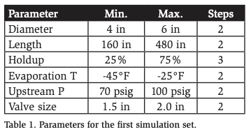
The first parametric simulation set consisted of 96 cases, implying 24 cases for each of the four geometries. The parameter ranges and the discretization setups used is shown in Table 1.

Quantities Extracted from Simulations

A post processing tool was developed that would automatically extract the following quantities from the different simulation folders of a parametric simulation set,

• The shock pressure and the time of occurrence of the shock after the hot gas injection was started 
• Slug detection and characterization in terms of, time to slug formation, slug velocity (front, back, average), and slug Joukowski number

The post processing tool would directly write out an Excel data file with the input and output columns.

Qualitative Results

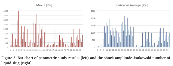
Some qualitative results obtained from the first simulation set is presented here. Bar graph of all the actual shock amplitudes is compared to the predicted slug Joukowski numbers in Figure 2. It is seen that the Joukowski predictions (right) are not as noisy as the shock amplitudes (left).

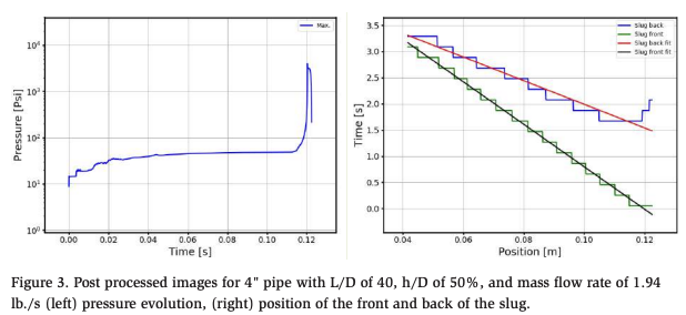
The output of the postprocessing script for the 4″ pipe with L/D of 40, h/D of 50% and mass flow rate of 1.94 lb/s is shown in Figure 3. Such graphs are available for each simulation run, however the postprocessing script goes further and extracts the shock amplitude and Joukowski numbers directly. The figure on the left shows the variation in the pressure in the piping with time. The maximum value is taken as the shock amplitude. The figure on the right shows the front and back of the slug as it travels towards the end cap. This is used to estimate the Joukowski number.

If no slug is formed the slug detection algorithm, which uses the liquid coverage of the pipe cross-section above 99% as the criterion, returns the information that a complete slug was not formed. With this information it can be decided whether the maximum pressure is a shock or just a pressurization of the system due to the hot gas entering. It was found that there was a total of 4 cases where the slug detection algorithm failed to detect a slug. The cases where slug formation was not observed were all for the 6″ pipe for an h/D of 25% and lowest two values of mass flow rates, viz. 0.31 and 0.48 lb./s.

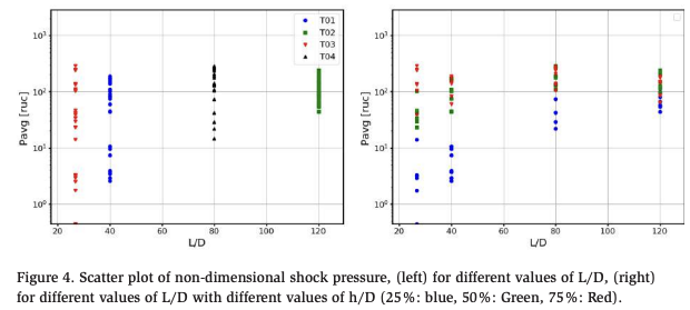
Effect of L/D and h/D

Interesting observations on the effect of the length of the pipework could be made by plotting the results. Figure 4 (left) shows the predicted non-dimensional shock amplitudes for each of the four setups, where L/D values of 40 and 120 are for 4″ pipes and L/D values of 27 and 80 are for 6″ pipes. For both diameters one can notice that as the L/D increases the height of the scatter reduces, implying that those cases that had lower shock amplitudes have shown higher shock amplitudes when the pipes are longer. We can conclude that the higher the L/D the more chances that a shock will occur. Figure 4 (right) shows the same values but colored differently for different values of h/D. Here we can see that the higher the h/D the higher the shock value for all setups. However, once there is sufficient liquid, the h/D = 50% gives marginally higher shock values. 

Parametric Set: -5°F

The initial dataset was extended by considering another temperature (-5°F) so as to allow a reasonable coverage of typical evaporation temperatures. The additional evaporation temperature of -5°F resulted in an additional 48 simulations for the same set of pipe diameters (4″ and 6″) and other parameters such as L/D, hot gas mass flow rates and liquid depths. For the chosen parameters, the shock amplitudes are expected to be significantly lower for the higher evaporation temperature. For the evaporation temperature of -5°F, seven cases were observed to not have slug formation and 17 cases had a shock amplitude below 250 psia. In total, therefore, 24 cases were observed to have a shock amplitude lower than 250 psia.

Parametric Set: 2″ Pipe

A set of simulations were performed for 2″ pipes. In this case, the h/D was fixed to 50% because the highest shocks were observed for this liquid level (see Figure 4). The L/D values were chosen to better cover the parametric space, resulting in the choice of 60 and 100. Only one value of evaporation temperature at -45°F and hot gas inlet temperature at 38°F were chosen. In the first parametric study the mass flow rate axis was sparsely discretized with only four values. For the 2″ pipe, 8 values of mass flow rates were chosen so that the dependence on mass flow rate is captured more accurately. This resulted in a total of 16 simulations, 8 for each value of L/D. The parameters for the 2″ pipe simulations are summarized in Table 2.

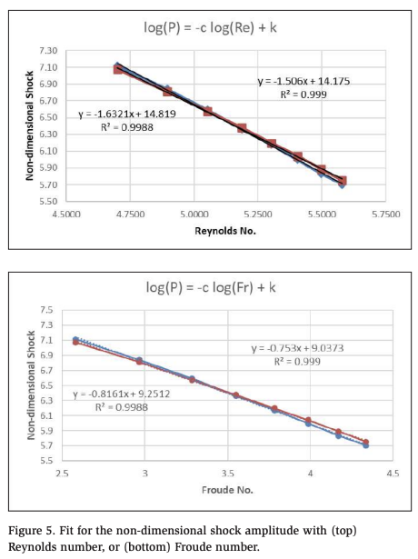
A more detailed analysis of the results for the 2″ pipe case was performed mainly to look at the effect of mass flow rate. In this case, the h/D, (pe, Te), and the inlet temperature, are constant and the only variables are L and mass flow rate. The non-dimensional numbers changing for different cases in this set are L/D, Re, Fr, System pressure to dynamic pressure (SPDP), and Mach. However, the four processdependent non-dimensional numbers are equivalent since only one parameter, i.e., the mass flow rate is varying. Therefore, one can envision a correlation for the non-dimensional shock pressure given as f(Fr, L/D) or f(Re, L/D) by restricting our attention to either Re or Fr.

The non-dimensional shock amplitude plotted against Re, and Fr is presented in Figure 5. A very good linear fit is obtained for the logarithm of the quantities. Only a very small difference is observed with respect to L/D. It is noted that the exponent is different by a factor of two because Reynolds number is linearly dependent on inlet velocity, whereas the Froude number depends on the square of the inlet velocity. The fit clearly shows that the non-dimensional shock amplitude is proportional to Re3/2.

Effect of Inlet Temperature

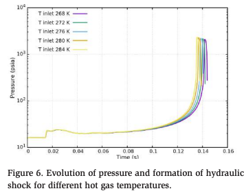
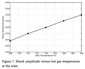
A small set of 4 simulations were performed to understand the impact of the hot gas inlet temperature on the shock amplitude. The 4″ pipe with L/D = 40, h/D = 50%, evaporation temperature = -45°F, and mass flow rate = 1.94 lb/s was chosen. The base case had a hot gas inlet temperature of 37°F. Four additional simulations with hot gas inlet temperatures of 23°F, 30°F, 44°F, and 52°F were performed. The pressure evolution and shock formation for the five cases are shown in Figure 6. A systematic influence of the hot gas temperature is observed, with the shock amplitude increasing with an increase in the inlet gas temperature. The variation of the shock amplitude against the inlet temperature is shown in Figure 7.

For the given conditions, the shock amplitude shows a rise of 13 psia/K of temperature rise. This shows that the non-dimensional number SPSH (system pressure to sensible enthalpy) should be retained in deriving the correlation for the shock pressure as a function of the relevant non-dimensional numbers. If the temperature is higher, the inlet gas density is lower and correspondingly the inlet velocity is higher for a given mass flux. Since the shock amplitude increases with increasing inlet velocity; this implies that the shock depends non-linearly on velocity (higher exponent than the density).

Correlation for Shock Amplitude

Based on the simulation-based dataset generated, a correlation for the shock potential (Joukowski number of the liquid slug) was developed. In total, 164 cases were simulated as described in the preceding sections. The first correlation was developed considering the whole dataset and a second one considering only the cases with h/D = 50%. This was done because when applying the correlation to a real case, the h/D would be unknown and therefore only the more serious case of h/D = 50% was considered. Results from the latter correlation are presented in the following sections.

Linear regression of the non-dimensional shock potential with respect to the five non-dimensional numbers was attempted. The following non-dimensional parameters were considered

1. L/D
2. Reynolds
3. Froude
4. SPDP (System pressure to dynamic pressure)
5. SPSH (System pressure to sensible enthalpy)

The linear regression was setup as follows,

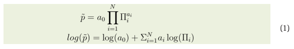
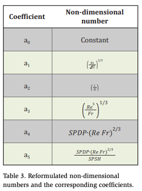
Where, p ~ is the non-dimensional shock pressure. The non-dimensional numbers used in the above formula were reformulated so that each number represented predominantly one of the input process or geometric parameter. The shock pressure was non-dimensionalized using the liquid density, liquid speed of sound, and the inlet gas velocity for the given conditions. The exponents (ai ) corresponding to the non-dimensional numbers (Pi ) are shown in below.

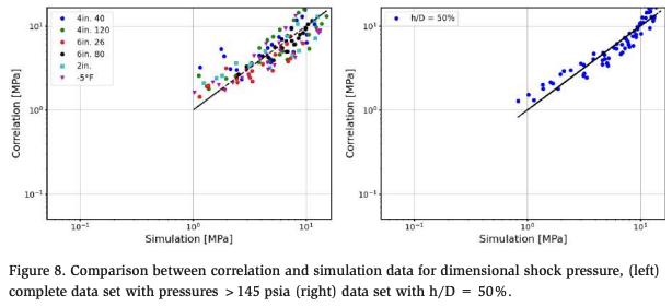
The correlation using only h/D = 50% data points, results in a very good fit with a regression score of 0.96. The correlation between the predictions from the fit and the simulation data is 98%. This indicates that the data points clearly represent an underlying physical behaviour and also that the form of the correlation (Eq. (1)) is appropriate to represent this behaviour. The scatter plot for h/D = 50% fit is shown in Figure 8 (right). A total of 67 cases were available for this fit.

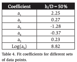
The coefficients of the fit are presented in Table 4. The following inputs are required to use this correlation,

• Diameter of pipe
• Length of pipework
• Evaporation temperature
• Hot gas mass flow rate
• Hot gas inlet temperature
• Properties database such as CoolProp (Bell, Wronski, Quoilin, & Lemort, 2014)

Critical mass flow rate to prevent slug formation

Before looking at applying the above correlation for different conditions, it must be reiterated that the correlation is only valid for conditions where the mass flow rate is large enough to form a liquid slug. The cases in the dataset where no slugs were formed were not considered in the correlation. Therefore, the correlation is not valid in the range where the flow rate is below the critical mass flow rate that is capable of inducing the transition from stratified to slug flow. This is the missing piece in the puzzle if it is desired to completely eliminate the risk of hydraulic shock from refrigeration systems. The formation of a slug or rather the transition from a stratified to a wavy flow is modeled by the Taitel-Dukler correlation for a pipe which is open (possibility for gas inflow and outflow with no pressure build up). For a rectangular cross-section, the Taitel-Dukler critical Froude Number ( * jG ) is given by,

where α is the fraction of the pipe cross-section occupied by the gas. The critical velocity of wave formation (and eventual slugging) expressed in terms of the critical Froude number is given by,

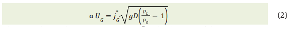
where g is the acceleration due to gravity, D is the diameter of the pipe, ρG is the vapor density, and ρL is the liquid density. The actual vapour velocity through the cross-section can be calculated as,

is the hot gas mass flow rate, and A is the cross-sectional area of the pipe.

The Taitel-Dukler (TD) correlation provides a critical velocity above which slugging occurs for a pipe that has stratified flow but not closed on one end. It is noteworthy that in the ASHRAE RP 970 experiments (Martin, Brown, & Brown, 2007), Martin et al. presented a modified form of TD correlation based on their experimental results because the TD correlation based on the inlet gas superficial velocity underestimated the critical velocity observed in the experiments. In other words, a much higher inlet superficial velocity was required in the experiments to create a slug as compared to the prediction of the TD correlation for an open (inflow-outflow) pipe. The modified correlation was given as,

Therefore, the critical mass flow rate above which slug formation can be expected can be estimated as,

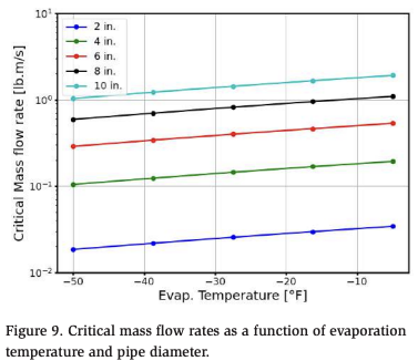
The critical mass flow rate from Eq. (16) is plotted in Figure 9 as a function of evaporation temperature for pipes of diameters ranging from 2″ to 10″ for fixed hot gas inlet temperature of 26°F. The predicted value for the critical mass flow rate for a 4″ pipe is approximately 0.1 lb./s and for a 10″ pipe is approximately 1.0 lb./s. These values seem to be reasonable. For the accident scenario simulated by Narayanan et al. (Narayanan, Wiencke, & Loyko, 2021), where the pipe diameter was 10″, the shock amplitude for 1.0 lb./s hot gas flow rate was small. The 4″ pipe simulations performed in this study had higher mass flow rates and slug formation was always observed—at least not contradicting the predicted critical mass flow rate.

Application of Correlation

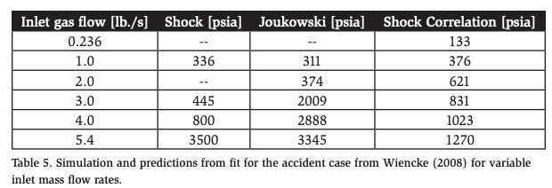
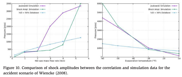
The correlation developed in the previous section is applied to the accident scenario simulated by Narayanan et al. (Narayanan, Wiencke, & Loyko, 2021). Note that the geometry of the piping in this case is quite different due to several bends, and the presence of a preformed slug above a liquid trap that was full. In that study, CFD simulations with the same modelling used here were performed with variations in hot gas mass flow rate and evaporation temperature. The simulation results were comparable to the estimations from the forensic analysis of the accident reported by Wiencke (Wiencke, 2008). The shock amplitudes reported in that study as a function of the hot gas mass flow rate is presented in Table 5. At low flow rates the shock amplitudes were not varying smoothly, whereas the shock potential represented by the Joukowski numbers of the slugs was found to vary smoothly. The shock potential predicted by the correlation developed in this study is seen to be much lower than the simulation results (column 4 of Table 5).

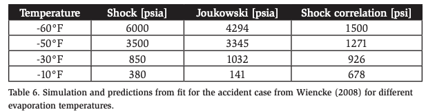
The shock amplitudes as a function of the evaporation temperature are reported in Table 6. A similar behaviour is observed for those cases, wherein the shock potential predicted by the correlations is significantly lower than the simulation data.

The same results are plotted in Figure 10 for the variation in mass flow rate and evaporation temperature. It is observed that the shock amplitudes predicted by the correlation are significantly lower than the simulations and also that the drop in shocking potential is slower for the correlation. The h/D = 50% correlation is good for the lower values and under-estimates the high shock values. This points to the fact that the correlation derived in this study, based on a scenario with a layer of stagnant liquid, would systematically predict lower shocks for the accident scenario where the liquid was already accumulated in the form of a slug in a trap. In the case where there is a layer of stagnant liquid all along the pipe the slug velocity would be lower since as the slug moves it comes into contact with a stagnant layer upstream.

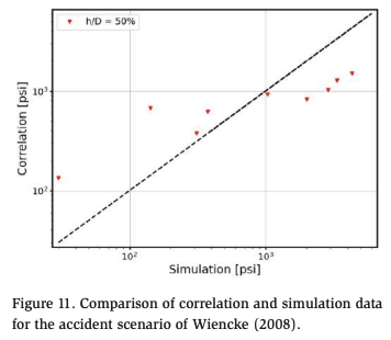
Scatter plot of the correlation prediction along with the simulation data for both sets of data is presented in Figure 11. Even though the values predicted by the fit are significantly lower, the correlation of the fit prediction to the simulation data is 92%.

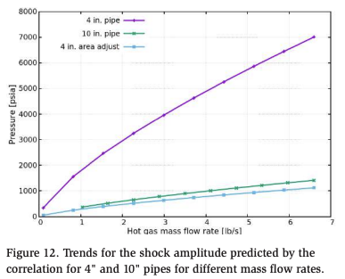
In order to further clarify the issue of the stagnant layer versus trapped liquid as discussed above, the fit is applied to 4″ and 10″ pipes for a range of mass flow rates comparable up to the high flow rate of 5.4 lb./s simulated for the accident scenario. An input deck to the correlation is created for 4″ and 10″ pipes with an L/D = 60 at an evaporation temperature of -50°F. The mass flow rate ranges from the critical mass flow rate for the given pipe diameter to 6.6 lb./s. The high flow rates maybe too high for the 4″ pipe but is used for the purpose of comparison to 10″ pipes.

The shock amplitudes predicted by the correlation is shown in Figure 12. It is seen that the shock amplitudes for the 10” pipe is much lower than the 4″ pipe due to the much larger cross-sectional area and other effects expected to be minor. The figure also shows that when the 4″ prediction is scaled down based on the area ratio between 10″ and 4″ pipes, it almost matches the 10″ shock predictions. This shows that the correlation behaves in a physically consistent manner. However, since the shock amplitude for the 10″ pipe in the accident scenario (Wiencke, 2008) for a mass flow rate of 5.4 lb/s is much higher, the different could be only due to the absence of a stagnant layer of liquid in the accident scenario.

Estimate valve opening time

In the study of motorized valves, it was found that even the introduction of a small opening time for the motorized valve resulted in very strong reduction in the shock amplitude. This was mainly because in all the instantaneous valve conditions simulated the time to shock formation was very small (less than 1 second). Therefore, as long as the opening time was greater than this time the shock amplitude was severely reduced. It was deduced that the motorized valve opening time should be much greater than the time taken for shock formation when using an instantaneous valve.

The time to shock formation could be predicted using the correlation developed above for instantaneous valve conditions. The method to do that would be to first predict the shock amplitude for required conditions. Since this shock value is actually the Joukowski number of the slug, the velocity of the slug can be estimated by dividing the Joukowski number by the liquid density and speed of sound at the evaluated at the evaporation temperature. Knowing the length of pipework and the slug velocity, the time to shock formation can be calculated. Apply a multiplicative factor so that the opening time is greater than the time to shock formation (could be an order of magnitude). For the accident scenario presented by Wiencke (Wiencke, 2008), the shock amplitude predicted by the correlation is 1,270 psia. This gives a slug velocity of approximately 23 ft/s and the corresponding time for the slug to reach the end cap as 2.5 s (for pipework length of 57 ft). Therefore, using the correlation and estimate of the minimum opening time of the motorized valve can be provided (10-25 seconds).

Summary for Fast-Acting Valves

In this section on instantaneous valves, a correlation has been developed to predict the shocking potential of an existing pipework for given hot gas mass flow rates, evaporation temperature, pipe diameter and pipe lengths. This correlation was shown to not give conservative predictions for situations not considered in this study such as the presence of liquid traps. The critical mass flow rate for slug formation, a prerequisite for downstream hydraulic shock, has also been presented. This correlation can be used, for example, for choosing a two-step valve such that for the first step the mass flow rate is chosen to be lower than the critical mass flow rate. In this way the study effectively addresses the issue of hydraulic shock prevention when using instantaneous valves.

Motorized Valves

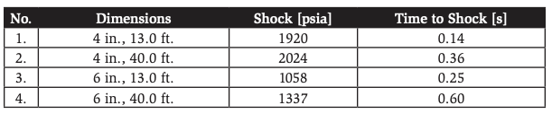
In order to study slow opening valves, one case from each setup in the first parametric study was chosen. In particular the cases with h/D = 50% and the highest mass flow rate for 4″ and 6″ pipes with different lengths. The valve characteristics studied were chosen from the product list of Danfoss. The specific parameters considered were h/D = 50%, Evaporation temperature = -25°F, hot gas inlet temperature = 38°F, and hot gas mass flow rate = 1.927 lb./s. The simulatio results for instantaneous valve opening from the parametric study is presented in

Table 7. All the cases chosen, show significant hydraulic shocks with the time to shock formation varying from 0.14 to 0.6 s (significantly less than 1 second).

Table 7. Shock amplitude and time to shock for instantaneous opening for the four cases chosen.

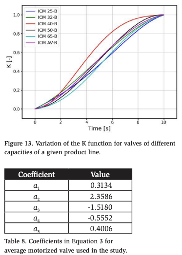
The transient mass flow rate of a motorized valve for given pressure difference is given in Equation (6). The factor K controls the mass flow rate as a function of the valve opening degree (Type-B valves from Danfoss).

where,

The variation of the K function based on the opening degree for different sized values of a certain type is shown in Figure 13. Since each valve has a slightly different characteristic, and therefore, the average K-factor as a function of opening time has been chosen. The coefficients for the K-factor used in this study are shown in Table 8. The coefficient a0 is not considered since the final mass flow rate is already known from the instantaneous cases chosen. 

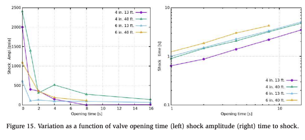
Simulations for each case were carried out for opening times of 1, 2, 4, 8, and 16 seconds. The pressure evolution for all four cases is shown in Figure 14. For all cases, the shock amplitude starts to reduce rapidly with an increase in the opening times. The shock amplitudes for all four cases are tabulated in Table 9. In all cases one can note that the shocks have become negligible at 16 seconds of opening time.

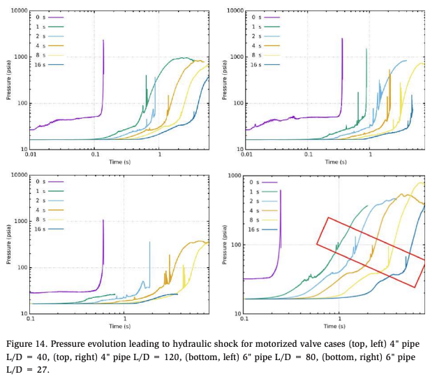
The main point to note is that for the cases where the time to shock for the instantaneous valve is much less than one second (the low L/D cases), the reduction in shock amplitude for one second of opening time itself is very significant. For the higher L/D cases, the reduction in shock amplitude happens at a larger opening time. This gives the hint that the opening time should be a function of both the mass flow rate as well as the length of the pipework so as to minimize the risk of large shocks.

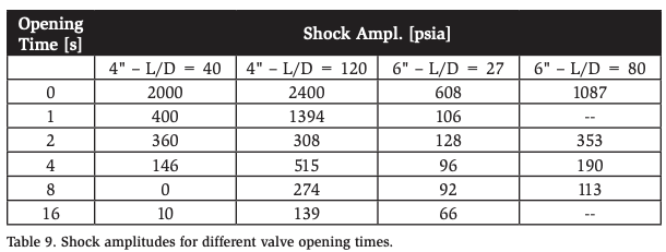
Table 10 presents the time for the occurrence of the shock for different opening times. As the opening time is increased the slug velocity is reduced thereby resulting in longer times for the occurrence of the shock.

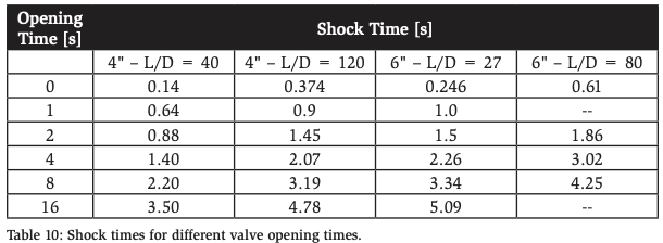
The shock amplitudes and shock times are plotted in Figure 15. Shock amplitudes go down very quickly with opening time and faster for the shorter pipes especially. The time to shock is seen to be a power law with the opening time.

Mesh refinement

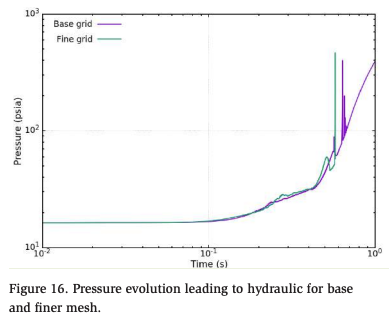
In order to gain further confidence on this remarkable observation on the potential of motorized valves to reduce and almost eliminate the possibility of hydraulic shock even at short opening times, one of the cases was simulated with a mesh that was two times finer in each direction. 

The case chosen was 4″ pipe, L/D = 40, -25° F, h/D = 50%, valve opening time of 1 sec. The fine mesh produced a shock of 466 psia in comparison to 400 psia for the base mesh. The instantaneous opening shock amplitude of 2000 psia is much higher than the difference due to a finer mesh; instilling confidence that this effect of the motorized valve is reliable. The pressure evolution for the base and fine mesh cases is shown in Figure 16.

Accident scenario of Wiencke (2008)

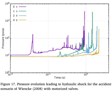
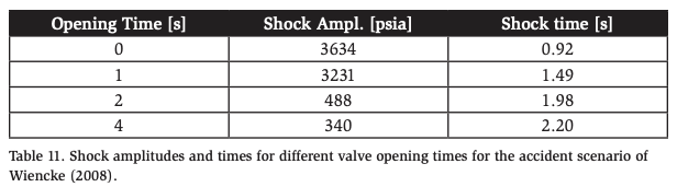
The accident scenario analyzed by Wiencke (Wiencke, 2008) was simulated with opening times of 1, 2, and 4 seconds for the hot gas mass flow rate of 5.4 lb/s. As discussed earlier, this case results in a shock of 3500 psia (refer to Table 5) for an instantaneous valve opening with a time to shock of approximately 0.9 seconds (Narayanan, Wiencke, & Loyko, 2021). The pressure evolution leading to hydraulic shock for different valve opening times is shown in Figure 17 with numerical values presented in Table 11. Results show reduction in shock amplitude; however, the reduction is minimal for an opening time of 1 second. For an opening time of 2 seconds the shock amplitude has already reduced by a factor of 6. This confirms the earlier observation that the valve opening time should be significantly larger than the shock formation time for the case of an instantaneous valve. It is expected that at an opening time > 10 seconds, the amplitude of the shock would be negligible.

This points to the possibility of using the correlation developed for instantaneous valves in this study to estimate the opening time for motorized valves. The method to do that would be to first predict the shock amplitude for required conditions. Since this shock value is actually the Joukowski number of the slug, the velocity of the slug can be estimated by dividing the Joukowski number by the liquid density and speed of sound evaluated at the evaporation temperature. Knowing the length of pipework and the slug velocity the time to shock formation can be calculated. Apply a multiplicative factor so that the opening time is greater than the time to shock formation (could be an order of magnitude). For the accident scenario presented by Wiencke (Wiencke, 2008), the shock amplitude predicted by the correlation is 1270 psia. This gives a slug velocity of approximately 7 m/s and the corresponding time for the slug to reach the end cap as 2.5 s (for pipework length of 17.5 m). Therefore, using the correlation and estimate of the minimum opening time of the motorized valve can be provided (10-25 seconds).

In summary, a remarkable observation was obtained by applying slow opening valve conditions to select cases from the parametric study. The shock amplitude goes down rapidly with finite valve opening time as long the opening time was significantly longer than the slug travel time for the given conditions. It leads to the conclusions that use of motorized valves could result in minimizing the risk of hydraulic shock with opening times still being very small compared to the hot gas process time scale. A method of estimating a safe opening time using the correlation for prediction of the shocking potential has also been proposed.

Conclusions

The study considered both fast acting and motorized valves. A correlation for the shock amplitude was developed as a function of process parameters using the simulation database. The fit had a very high regression score and correlation to the source data. This fit could be directly used to assess the hydraulic shock risk in current refrigeration systems which use single-step or two-step fast acting valves. The critical mass flow rate below which the formation of a liquid slug by the hot gas flow has also been presented. This correlation gives an upper limit on the mass flow rate for fast acting valves if hydraulic shocks are to be prevented. Finally, simulations of motorized valves for different opening times have shown that valve opening times greater than the system length divided by the average slug velocity will significantly reduce the potential shock pressures. This system time scale can be directly estimated from the correlation developed in this study for the shock amplitude as a function of process parameters. Based on these results, this study could be used to lay the foundation for new design guidelines in the future.

Putting all the pieces together:

1. The use of motorized valves with sufficiently long opening times mitigates any risk for hydraulic shock.
2. Higher values of L/D result in higher shock amplitudes.
3. Shock amplitudes diminish in value as the evaporating temperature increases.
4. The highest shock amplitudes occur when the liquid level h/D is between 25% and 75%.
5. The modified Taitel-Dukler correlation due to Martin et al. (2007) provides the critical hot gas mass flow rate above which slug formation and hydraulic shock can occur.
6. A correlation has been developed to predict the hydraulic shock amplitude in an existing pipework for given operating conditions.
7. This correlation can be also used to estimate the opening times of motorized valves that would prevent hydraulic shocks.

Acknowledgements

The authors gratefully acknowledge the research funding provided by the ARF and the contributions of the PMS for their inputs and constant interest, guidance, and encouragement. Special thanks to Bent Wiencke for his leadership in steering the project. We also acknowledge the contributions of the AMS group of AFRY Switzerland for the support and resources to conduct this work.

References

Bell, I., Wronski, J., Quoilin, S., & Lemort, V. (2014). Pure and pseudo-pure fluid thermophysical property evaluation and the open-source thermophysical property library CoolProp. Industrial & engineering chemistry research, 53(6), 2498-2508.

Labois, M., & Narayanan, C. (2017). Non-conservative pressure-based compressible formulation for multiphase flows with heat and mass transfer. International Journal of Multiphase Flow, 96, 24-33.

Martin, C., Brown, R., & Brown, J. (2007). Condensation-Induced Hydraulic Shock, Final Report, Tech. Rep ASHRAE 970-RP. ASHRAE.

Narayanan, C. (2021). Numerical simulation of flashing using a pressure-based compressible multiphase approach and a thermodynamic cavitation model. International Journal of Multiphase Flow, 135, 103511.

Narayanan, C., Thomas, S., & Lakehal, D. (2020). CFD Study of Hydraulic Shock in Two-Phase Anhydrous Ammonia. ASHRAE Transactions, 126.2.

Narayanan, C., Wiencke, B., & Loyko, L. (2021). CFD Analysis of Pipework Fracture due to Hydraulic Shock in an Ammonia Refrigeration System. IIAR Natural Refrigeration Conference & Expo. Palm Springs, CA, USA: IIAR.

Saurel, R., & Lemetayer, O. (2001). A multiphase model for compressible flows with interfaces, shocks, detonation waves and cavitation. Journal of Fluid Mechanics, 431, 239-271.

Van Doormaal, J., & Raithby, G. (1984). Enhancements of the SIMPLE method for predicting incompressible fluid flows. Numerical heat transfer, 7(2), 147-163

Wiencke, B. (2008). A Case Study of Pipework Fracture due to Hydraulic Shock in an Ammonia System. IIAR Ammonia Refrigeration Conference & Exhibition. Technical Paper #6. Colorado Springs, Colorado, USA: IIAR.

Zhu, J. (1991). A low-diffusive and oscillation-free convection scheme. Communications in applied numerical methods, 7(3), 225-232.